Robot Arm Motion Profiler
A motion profiler for a two degree of freedom robot arm. Personal Project
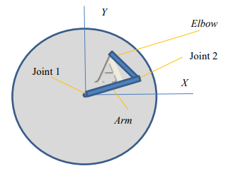
For a final project a professor challenged us to design a two-dimensional, two degree of freedom robotic arm that would allow for automated machining of precise shapes. Namely two letters of the alphabet must be chosen and placed within the quadrants surrounding the first joint (Figure 1). For these letters a path must be chosen and all kinematics and kinetics of both arms must be graphed.
Our criteria were as follows:
- Constant speed during “active” regions (parts where the end effector is in use to make the letters)
- Must start and end operation at a designated home position
- Instant acceleration cannot occur so an acceleration region must be made before each segment of a drawing
- Design of arm must include motor choice that matches requirements of trajectory path chosen and the kinematics and kinetics required (torque)
- A comprehensive explanation of the system/robot design.
To complete the outlined goals, a path must be defined in 2D Cartesian space that our robot will follow. To do this a SVG image is decoded and converted to the (X,Y) coordinate space. Through this decoding we find lines and curves to match the input image and define way points along this path to mark where the end effector should move to. Instead of hard-coding for a specific task, decoding SVG images allows for utmost flexibility and rapid iteration of designs and greatly improves the effectiveness of the robot and allows us to display any letter with ease as well as any basic image.
To construct a motion profile where we have a constant velocity along curves and a maximum acceleration value we need to know the distance needed to accelerate our end effector to the desired speed before it hits a curve. We decided to use Python and generalize our code to work with any SVG drawing made of lines and cubic Bezier curves.
We decode the SVG, getting equations of lines we want to draw. We can then use simple kinematics to obtain the distance we need to accelerate to the desired speed.
By taking the derivative of the ends of the curves we can identify the direction we need to be accelerating in. We can then use the accelerationDistance to know how far from the point we have to be. Using this information, we can make a motion profile from these acceleration points to the start of any curve.
Maintaining a constant velocity on a curve is relatively simple task on a straight line, using this formula:
When Velocity and time are already known, simply move a set distance per “frame” (set unit time). The problem becomes more complicated when dealing with cubic Bezier curves. Determining the arc length of these curves is very difficult. After trying a variety of methods, I settled on a numerical method of approximating the curves by estimating them as a large number of small straight lines. This method works well but accumulates error that at the end of the curve will cause unacceptable “jumps” in velocity and acceleration values. Because of this the approximation has to be very accurate resulting in ~320000 lines being used to approximate an average sized curve. With this accurate approximation of arc length we can use our formula to know that we need to travel a certain distance over the curve for a set amount of time.
To connect the ends of the acceleration points together we need a third movement type that will not activate the end effector and also does not need to have a max speed. To achieve the fastest line the end effector must be accelerating for half the time and decelerating for the other half of the time.
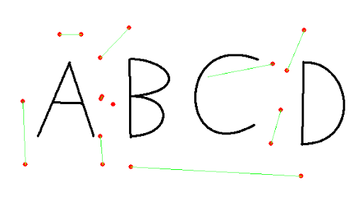
Figure ABCD shows an exaggerated view of how our program calculates the trajectory. The red dots are the points we begin accelerating at to achieve the desired velocity at the black lines. The green lines are our moves that connect those red dots.
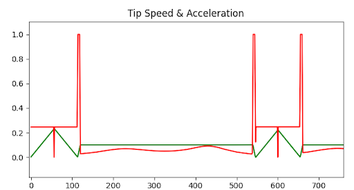
Figure 8 shows an example of 3 moves. The 2 triangular movements correspond to the green lines in Figure 7 where speed does not matter and the goal is to get to the next acceleration point. This move has ¼ the acceleration to ensure that the speed does not cause a torque value too high for our motors. The trapezoidal movement is before, during and after the line demonstrating constant velocity while on the line and a maximum acceleration that is set in code during the acceleration and deceleration period. The repository for this project can be found here.